A bubble chart puts two numbers on the axes and a third in the area of each circle. Use it when that third measure changes how the audience should read the comparison. Keep each bubble tied to one row, explain the size scale, and size circles by area: a value four times larger needs twice the radius, not four times the radius.
For a broader choice of visual, the guide to chart types for presentations helps you decide whether three measures belong in one view. Below, a six-queue support example shows how to build a readable bubble slide, check its arithmetic, and explain what it does—and does not—establish.
When does a bubble chart help?
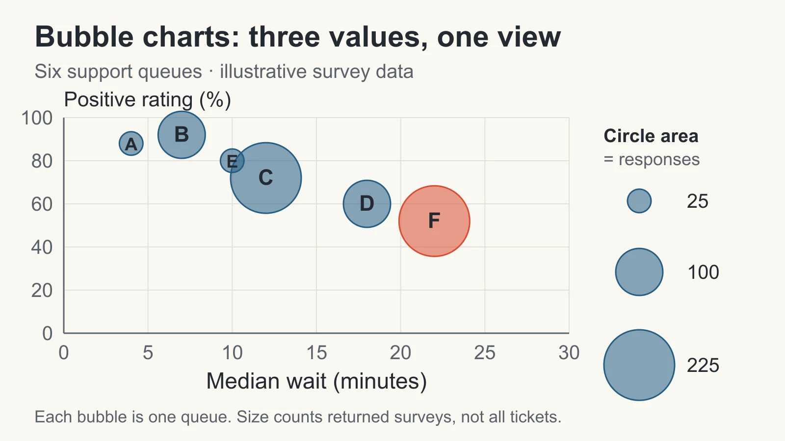
A plain scatter plot is enough when the question concerns two numeric measures. A bubble chart adds useful context when the magnitude behind each point matters too: for example, waiting time and satisfaction alongside the number of survey responses. Microsoft’s bubble-chart documentation describes the three inputs as x, y, and size values; both axes are numeric.
Before adding size, finish this sentence: “Knowing the third value changes our discussion because ___.” In the example, a low rating based on 225 returned surveys deserves a different follow-up from a low rating based on 25. That does not make the larger group automatically more representative or statistically conclusive. It tells the audience how much recorded feedback sits behind the point.
Use bars or a table when the main task is ranking exact amounts. Use a scatter plot with equal-size markers when the third measure adds no useful distinction. Avoid using circle sizes to encode category names, negative balances, or an undefined notion of “importance.”
Prepare one row for each bubble
This is an illustrative dataset, not customer research. Imagine six support queues over the same reporting week. Each row describes customers who returned a survey after their interaction. Waiting time is the median for those respondents, positive rating is their share selecting a positive response, and bubble area represents their number of completed surveys.
| Queue | Median wait (min) | Positive rating | Surveys (n) |
|---|---|---|---|
| A | 4 | 88% | 25 |
| B | 7 | 92% | 100 |
| C | 12 | 72% | 225 |
| D | 18 | 60% | 100 |
| E | 10 | 80% | 25 |
| F | 22 | 52% | 225 |
For A, 22 positive responses out of 25 give 88%. For F, 117 out of 225 give 52%. Those counts make the percentages traceable. Keep the underlying response records with the working file; the median cannot be reconstructed from this summary table alone.
Use the same population and reporting window for all three values. If waiting time covers every ticket but ratings cover only respondents, label the difference explicitly and decide whether the combined view still answers the question. A neat chart cannot repair a mismatch in what its measures describe.
Scale the area, not the radius
A circle’s area is πr². To make area proportional to a positive value, calculate the radius using its square root. If a 25-response bubble has radius 12 pixels, use:
Radius = 12 × √(responses ÷ 25)
The radii for 25, 100, and 225 responses are therefore 12, 24, and 36 pixels. Their areas have the correct ratio of 1:4:9. These pixel sizes are a construction example; resize the whole set together to fit your slide.
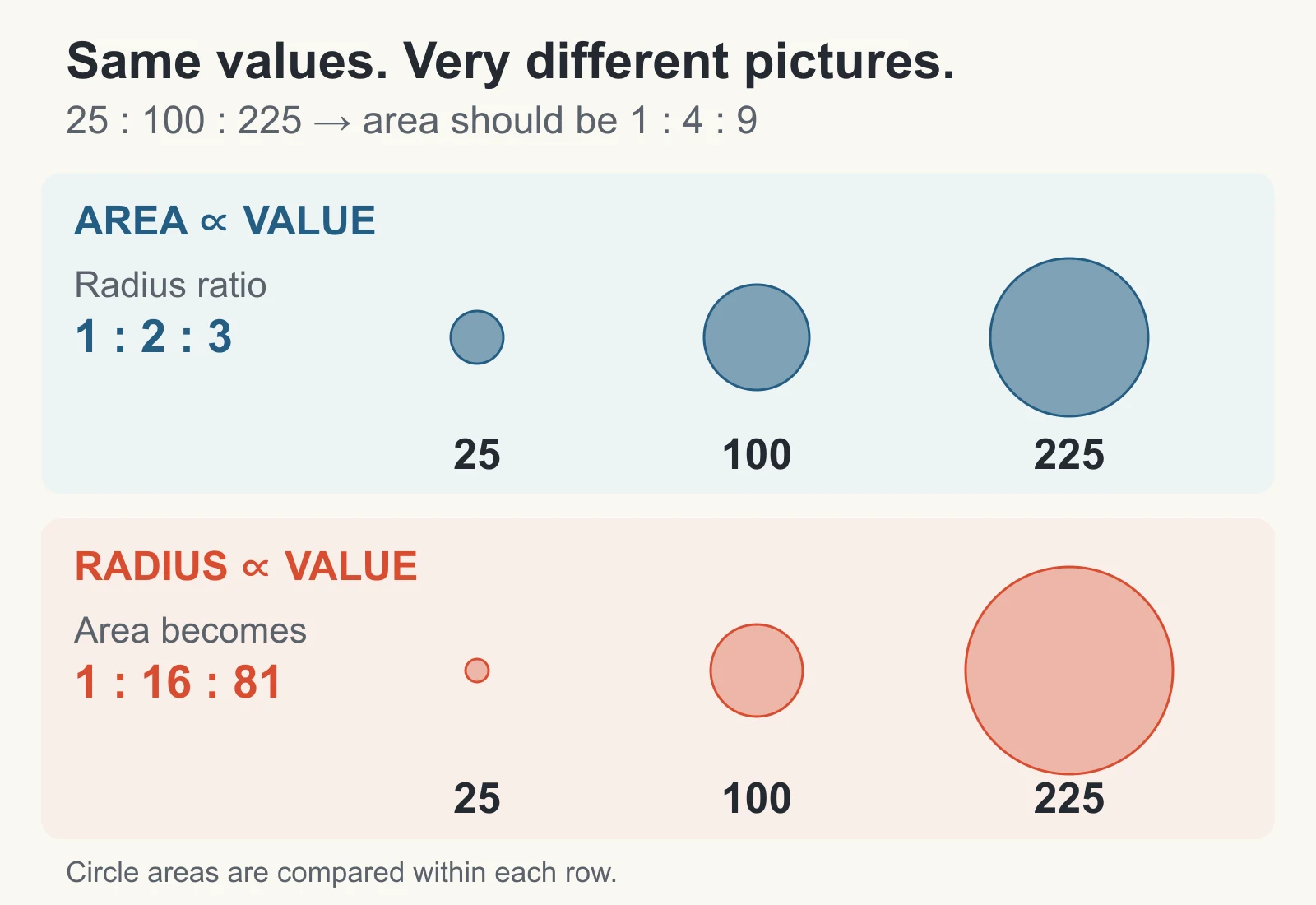
If you instead multiply the radius by four for 100 responses, its area becomes 16 times the 25-response circle. A ninefold radius for 225 responses creates 81 times the area. The biggest group then looks much more dominant than the data supports.
In a chart tool that asks for a size column, supply the original values—25, 100, 225—not square roots you calculated for manually drawn radii. Check the tool’s size settings and the result. Transforming values first when the tool already scales areas would apply the adjustment twice.
Include a size key with labeled circles, such as 25, 100, and 225 responses. Keep it on the same scale as the plot. If you compare several slides, keep both the size scale and axis bounds consistent; independent automatic scaling can make an unchanged quantity look larger on the next slide.
Build and check the slide
- Map the three measures explicitly. Use median wait for x, positive rating for y, and survey responses for size. Keep queue IDs with the rows. In Excel, place the numeric x, y, and size columns together and choose a bubble chart from the scatter-chart group; confirm the series ranges afterward.
- Use a flat chart with visible axes. For this example, a 0–30 minute x-axis and 0–100% y-axis leave room around the marks. State both units. The bubble centers carry the coordinates; circle edges do not represent ranges or uncertainty.
- Verify three rows before styling. A must sit at (4, 88) with size 25; C at (12, 72) with size 225; F at (22, 52) with size 225. C and F must have equal areas even though their positions differ.
- Make the marks readable. Use one restrained color and highlight the queue being discussed. An outline and partial transparency can help reveal overlap. Add labels or leader lines where needed; do not move a bubble away from its actual coordinates to make room.
- Carry the definitions with the chart. Keep the period, population, units, size key, and source note on the slide or in an accompanying readable note. Preserve the source table for questions and updates.
A 3-D effect adds no fourth measure here and can make sizes harder to compare. Similarly, a bubble’s apparent prominence should come from a documented value or a clearly explained highlight, not a shadow or glow.
Keep the percentage scale consistent. The example’s plotting values use 88 to mean 88%, so the y-axis runs from 0 to 100 with a percent label. If you enter 88% in Excel, the stored value is 0.88; use bounds of 0 to 1 and percentage formatting instead. Do not apply percentage formatting to a stored value of 88, which would display as 8,800%, or mix these two conventions within one series.
Write a takeaway the chart supports
A useful headline for the example is “Queue F combines a long wait, a low rating, and 225 survey responses.” It identifies a concrete follow-up without pretending the chart explains the cause.
You could say: “F’s respondents waited a median of 22 minutes, and 52% gave a positive rating. Its 225 responses give us a substantial feedback group to investigate. We should review the queue’s case mix and any accompanying survey comments before deciding what to change.” This is a proposed next action for the fictional scenario, not a tested improvement; the summary table does not contain comments.
Avoid “Waiting longer caused poor satisfaction” or “F is our worst service team.” These are six aggregate observations from survey respondents. Case complexity, response patterns, staffing, and other differences have not been accounted for. The chart also does not show the total number of customers served: response count and ticket volume are different measures.
Handle overlap, zero values, and missing sizes
When bubbles overlap: reduce their overall size while preserving area ratios, use transparency, or split the chart into small multiples with shared scales. If two queues have identical coordinates, name both in an annotation or provide a separate detail view. Do not silently add their response counts unless a combined group is meaningful and its x and y values have been recomputed from the underlying data.
When the size is zero: a proportional bubble has zero area and will disappear. If visibility matters, use a separate zero-value symbol with an explicit legend. In this survey example, zero responses also means the positive-rating percentage is undefined; the queue cannot be placed as an ordinary x-y-size observation.
When the size is missing: keep it distinct from zero. Identify the excluded queue and the missing measure in the note, then seek the source value. Do not use a decorative default radius that looks like a measured count.
When values can be negative: circle area cannot carry a negative quantity directly. Use another chart, or separate magnitude and sign with a clearly documented encoding. Do not turn a negative value positive without explaining what changed.
Turn the checked chart into a presentation
Once the data mapping is settled, use Presenti’s text-to-presentation workflow to draft the explanation around it. Provide the audience, takeaway, measure definitions, and the question the team should investigate. Check the generated wording against the table.
A practical brief is: “Create a short presentation for a support review. Explain the six-queue survey example, define waiting time and positive rating, and identify questions to investigate about Queue F. Label every example value as illustrative. Do not invent causes, statistical tests, or improvement results.”
Prepare and verify the bubble chart in a charting tool with explicit x, y, and size controls. This workflow does not rely on Presenti providing a native bubble-chart type. Keep a checked chart file and its source table with the deck, and verify its appearance after placing it in your chosen presentation editor. A static chart image can preserve the visual, but it does not preserve editable chart data.
Before presenting, show the slide at its actual viewing size. A listener should be able to identify what one bubble represents, what each axis measures, what size means, and which conclusion is supported. If that explanation takes longer than the point you are making, simplify the chart.